A Gentle Introduction to Singular Learning Theory

I’ve been reading about Singular Learning Theory (SLT) lately, a framework developed by the statistician Sumio Watanabe, and I wanted to write down what I’ve understood so far: partly to organize my own thoughts, partly because it’s one of the more interesting ideas floating around in the “why does deep learning even work” corner of ML theory. This post is a friendly overview, not a technical deep dive. If you’re starting a PhD and keep hearing “SLT” and “developmental interpretability” thrown around, hopefully this helps.

The problem with classical learning theory

Classical statistical learning theory makes a convenient assumption: models are regular. In plain terms, this means every distinct setting of the parameters gives a distinct probability distribution, and the loss landscape around the best parameters looks roughly like a smooth bowl, essentially a Gaussian. This is a nice assumption because it lets you do a lot of clean math around it.

Concretely, if $w_0$ is the true (best) parameter and $K(w)$ is the population loss (the KL divergence between the true distribution and the model’s distribution),

\[K(w) = \mathbb{E}_{x}\left[\log \frac{q(x)}{p(x \mid w)}\right],\]

then the regularity assumption says $K(w)$ is well approximated, near $w_0$, by a simple quadratic bowl:

\[K(w) \approx \frac{1}{2}(w - w_0)^\top I(w_0)(w - w_0),\]

where $I(w_0)$ is the Fisher Information Matrix (defined below) evaluated at $w_0$. This is exactly the Taylor expansion of a smooth, bowl-shaped function around its minimum, and it’s only valid if $I(w_0)$ is invertible. Invertibility is what makes the bowl curve upward in every direction: if $I(w_0)$ had a zero eigenvalue, the quadratic term would vanish along that direction, and $K(w)$ would stay flat there instead of curving up. It also underlies classical asymptotic theory more broadly, since the standard result that the maximum likelihood estimator is asymptotically normal, with covariance $I(w_0)^{-1}$, requires that inverse to exist.

The problem is that this assumption is basically false for almost every model we actually care about: neural networks, hidden Markov models, and so on. These models are heavily overparameterized: many different parameter settings can produce the exact same input-output behavior. The “bowl” assumption breaks down.

What makes a model singular

This is where Singular Learning Theory comes in. SLT studies exactly the case that classical theory ignores: models that have singularities, which are points in parameter space where the Fisher Information Matrix is degenerate.

A quick refresher on the Fisher Information Matrix (FIM): it measures how sensitive a model is to small changes in its parameters. If you nudge a parameter slightly, how much does the model’s output change? Formally,

\[I(w) = \mathbb{E}_{x \sim p(x \mid w)}\Big[\nabla_w \log p(x \mid w)\, \nabla_w \log p(x \mid w)^\top\Big],\]

i.e. the covariance of the score function (the gradient of the log-likelihood).

The FIM is degenerate, or non-invertible, when

\[\det I(w_0) = 0.\]

That means the matrix applies a transformation that can’t be undone: some information gets collapsed. Concretely, there exists some direction $v \neq 0$ with $v^\top I(w_0) v = 0$, meaning $K(w_0 + \epsilon v) \approx 0$ to second order. Practically, this shows up as singularities: parameter directions that don’t actually matter. In other words, you can move the parameters in these directions without changing the model’s behavior at all. These are the redundant, “invisible” directions of the model.

A sharp, bowl-shaped minimum (regular case, left) next to a flat, wide minimum (singular case, right). Optimization trajectories (red) settle much faster in the sharp bowl than in the flat one. Source.

Measuring complexity: the RLCT

If some parameters are redundant, then just counting the number of parameters is a bad way to measure a model’s real complexity. SLT instead uses a quantity called the Real Log Canonical Threshold (RLCT), usually written as λ. The RLCT captures the model’s true effective complexity: how much of the parameter space actually matters, geometrically, around a given point.

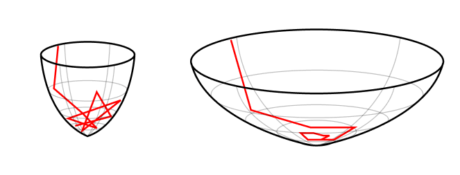
One intuitive way to define it: look at how the volume of “near-optimal” parameters shrinks as you tighten the loss threshold $\varepsilon$ around $w_0$,

\[\mathrm{Vol}\big(\{w : K(w) \le \varepsilon\}\big) \sim C\, \varepsilon^{\lambda} \quad \text{as } \varepsilon \to 0.\]

In the regular case, $K(w)$ is a $d$-dimensional quadratic bowl, so each of its $d$ axes shrinks like $\sqrt{\varepsilon}$ as you tighten the threshold, and the volume of that ellipsoid scales as the product of its axis lengths, $(\sqrt{\varepsilon})^d = \varepsilon^{d/2}$. That’s exactly why classical theory predicts $\lambda = d/2$, half the parameter count. In the singular case, the flat directions make the near-optimal region shrink more slowly as $\varepsilon \to 0$, so $\lambda < d/2$: a direct, geometric sense in which the model is “simpler” than its raw parameter count suggests.

This shows up in a quantity called the free energy, which we want to minimize. Intuitively, the free energy is the (negative log) Bayesian evidence for a region of parameter space: how strongly the data supports that region once you’ve paid a fair price for how much of the hypothesis space it occupies. A region with low free energy is one the data prefers, either because it fits well, because it’s geometrically simple, or some balance of both. Watanabe’s asymptotic formula for the (negative log) marginal likelihood over $n$ samples is:

\[F_n = n K_n(w_0) + \lambda \log n - (m - 1) \log \log n + O(1),\]

where $m$ is a multiplicity term (usually $1$) and $K_n(w_0)$ is the empirical loss at the optimum. Dropping the lower-order terms gives the simplified picture I’ll use for intuition:

\[\text{Free energy} \approx \underbrace{\text{fit to data}}_{\text{loss}} + \lambda \cdot \log(n)\]

where:

the fit to data term is just the loss (smaller means the model fits the data better),
λ (RLCT) is the effective complexity,
n is the sample size.

The intuition is nice once you see it. When λ is low, the loss landscape is flat around this region, so the effective complexity is low: a flat singularity. When λ is high, the landscape is sharp, so the effective complexity is high: a sharp singularity.

A flat region means there are directions around this optimum that don’t really matter, so the model, in some sense, is “simpler” than it looks, even if it has millions of parameters. Free energy formalizes the classic intuition that flatter minima tend to generalize better.

Why bother with SLT?

The main motivation is that SLT gives us a language to talk about strange deep learning phenomena that classical theory can’t explain: things like phase transitions, grokking, and double descent. These are all cases where a model’s behavior changes abruptly or non-monotonically during training, which doesn’t fit neatly into the “smooth bowl” picture at all.

That said, I should be honest: SLT is still not very practical, at least not yet. λ can be computed exactly for small toy models, but it’s intractable for anything the size of a real neural network. It’s linked to generalization performance, which is promising, but that connection isn’t fully worked out. Most of the vocabulary and theorems were built for Bayesian models, and extending them to networks trained with SGD is promising but still not rigorous. So far, SLT hasn’t produced concrete training improvements or architectural insights: it’s more of a theoretical lens than an engineering toolkit.

The link with developmental interpretability

This is the part I find most exciting. There’s a growing research direction called developmental interpretability (DI) that uses SLT as a lens for mechanistic interpretability (MI), but with a twist. Instead of just analyzing the final trained model, DI looks at how a neural network changes during training.

The name is a deliberate echo of developmental biology, the study of how a single fertilized cell turns into a fully formed organism through a sequence of developmental stages, rather than just how the final adult body is structured. DI borrows that framing: instead of asking what a trained network computes, it asks how the network’s internal structure unfolds over the course of training, one stage at a time.

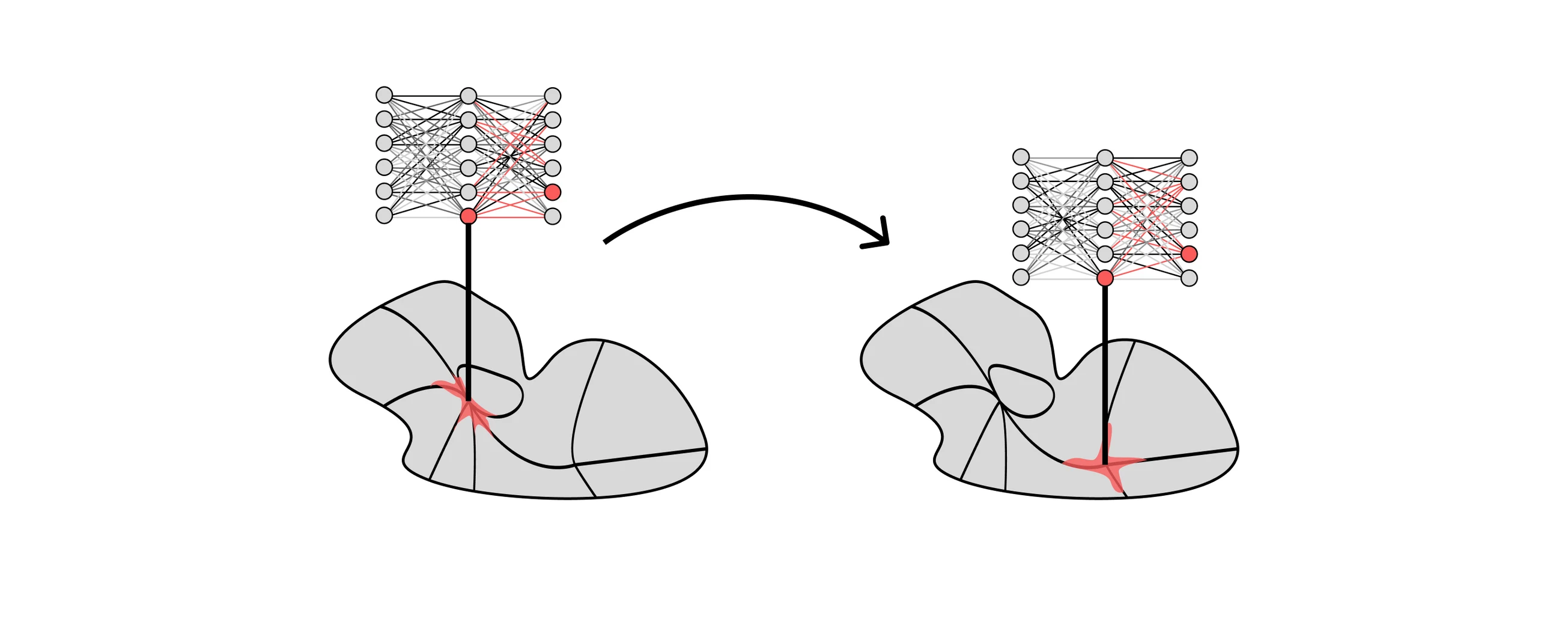
Here’s the connection to phase transitions: SGD can be thought of as moving between different singular regions of the loss landscape over the course of training. Each region roughly corresponds to a different “computational strategy” the network is using internally. A phase transition, then, is a sudden shift from one region (one strategy) to another.

This is a genuinely different question from what most MI work asks. Most MI research starts from a finished network and tries to reverse-engineer what it’s doing. Developmental interpretability instead asks: how does the network become what it is? It’s less about dissecting the final artifact and more about understanding the process that produced it.

As training progresses, the network's parameters move across the singular loss landscape, crossing from one singular region into another: a phase transition. Source.

Where things stand

Combining SLT and developmental interpretability is still a very young idea, more of a research program than an established field. There’s a real theoretical foundation (SLT has been around in the statistics literature for a while), but connecting it usefully to how we actually train and interpret large neural networks is very much a work in progress.

That’s part of what makes it appealing to me: the foundations are solid, but there’s clearly a lot left to figure out.

Additional sources

If you spot something inaccurate here, feel free to reach out. This is very much a “learning in public” post.