How Transformers Actually Work: From First Principles to Production

If you’ve used ChatGPT, Claude, or any modern language model, you’ve interacted with a transformer: it is simply a neural network architecture from 2017 that turned out to scale far better than anyone expected. This post is some kind of first tour for anyone learning about transformers: we start with the bare architecture, then walk through the tricks that turn a textbook transformer into something you can actually train efficiently and serve to millions of users cheaply.

The goal is not to be exhaustive, as entire papers exist on single ideas mentioned below. Instead we want to create a mental map: why each trick exists, what problem it solves, and how it works, with just enough math to make things concrete and clear.

Act I — The Shape of a Transformer

At the highest level, a transformer is actually pretty simple to describe: it’s a stack of repeated blocks, and each block does exactly two things, one after another: 1) attention, where tokens exchange information with each other, and 2) a feed-forward network (MLP), where each token’s representation is processed independently. So we roughly have:

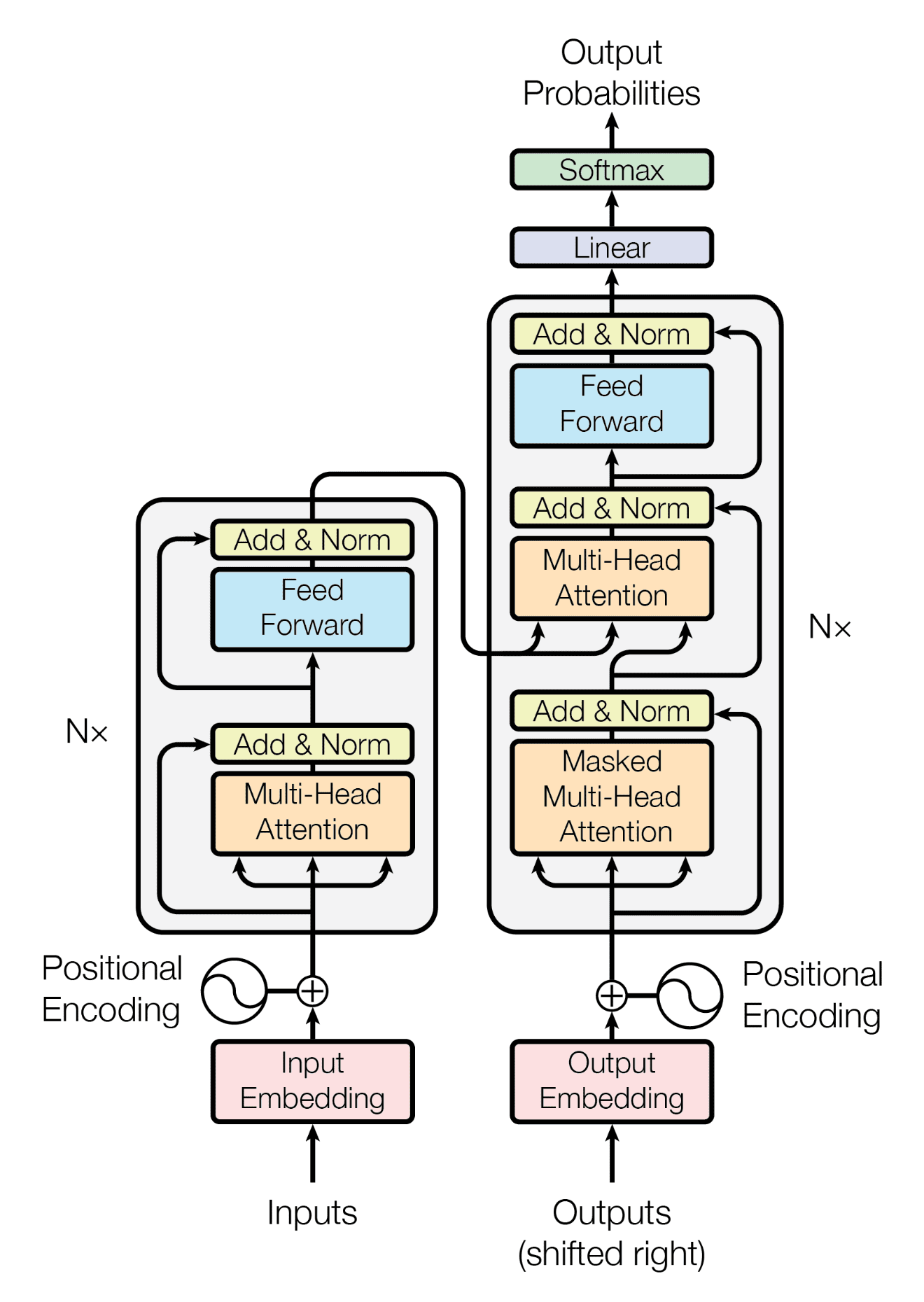
If we stack many of these blocks on top of each other, each layer will refine the representation of every token a little further: it sharpens ambiguous meanings, incorporates context from other words, and hopefully produces a representation rich enough to predict what comes next. Almost every fancy concept or trick about LLMs (KV caches, RoPE, Mixture of Experts, quantization, RLHF) is either a variation on how attention or the MLP is computed, or a system-level trick for making the training or serving of this stack faster and cheaper. Keeping that framing in mind makes the rest much easier to follow.

Attention: how tokens talk to each other

Attention is the mechanism that lets a token look at previous tokens and decide which ones are relevant, then pull information from them, which can be sen as a learned form of information retrieval. For every token, the model learns three different projections of its hidden vector $x$:

Query (Q) asks “what am I looking for?”, Key (K) answers “what information do I contain?”, and Value (V) answers “what should I pass along if I’m selected?”. A useful analogy is the library search: your query is the search string you type, every book’s key is its index card, and once you know which books are relevant, you don’t read the index card, you read the actual content, the value.

When token $A$ attends to token $B$, it compares $A$’s query against $B$’s key via a dot product, $\text{score}(A,B) = q_A \cdot k_B$. If the match is strong, $A$ attends more heavily to $B$ and pulls in more of $B$’s value vector. For a whole sequence, we compute a score between the current token and every previous token, $\text{scores} = q_{\text{current}} \cdot k_{\text{prev-tokens}}$, divide by $\sqrt{d_k}$ to keep the softmax that follows well-behaved (without this scaling, dot products in high dimensions grow large and push the softmax into a regime with vanishing gradients), and pass the result through a softmax so the scores sum to 1. The model then takes a weighted average of the value vectors using these softmax weights: this weighted average is the new information the current token receives about everything that came before it. Putting it together leads to the classic formula from Vaswani et al. (2017):

For a decoder-only model (the kind behind essentially all modern LLMs), a token is only allowed to attend to itself and earlier tokens, never future ones. This causal mask (implemented by setting future scores to $-\infty$ before the softmax) is what makes left-to-right generation coherent: token $n$ never had access to token $n+1$ during training, so there’s no mismatch with how the model is later used to generate text one step at a time.

A single attention computation captures one kind of relationship, but language has many simultaneous relationships to track like syntax, coreference, topic, sentiment… So transformers run many attention heads in parallel, each with its own $W_Q, W_K, W_V$, free to specialize in a different pattern, then concatenate all the heads’ outputs and mix them with one more learned projection:

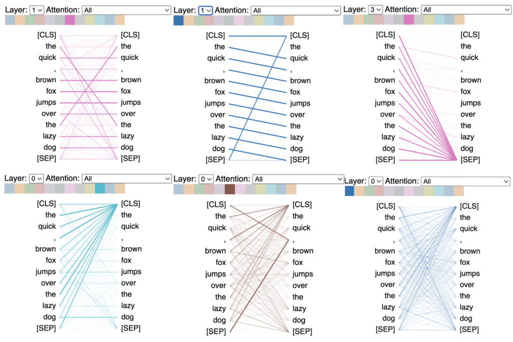
The MLP, residual streams, and normalization

After attention, each block has a feed-forward network. The difference with attention is quite clear: attention moves information between token positions, while the MLP processes information within each position. Structurally it’s a simple two-layer network applied identically to every position, $\text{MLP}(x) = W_2\,\sigma(W_1 x)$, with a hidden dimension typically 4x wider than the model’s embedding size (this is where a large fraction of the model’s parameters, and its capacity to store facts and patterns, actually lives).

Most modern LLMs (LLaMA, PaLM, Mistral, and others) don’t use a plain nonlinearity here, but a gated one, most commonly SwiGLU (Shazeer, 2020):

One linear projection acts as a gate controlling how much of a second projection passes through, elementwise. This costs a third weight matrix but consistently improves downstream quality for a comparable parameter budget, so labs shrink the hidden dimension slightly to keep total parameters roughly constant.

But how does information actually persist across all these blocks? Instead of each layer completely replacing the previous representation, every layer adds an update on top of it: $x_{l+1} = x_l + \text{Layer}_l(x_l)$. A useful picture, popularized by Anthropic’s interpretability work: each token has a persistent “shared workspace” vector — the residual stream — running through the whole depth of the network, which every attention head and MLP reads from and writes small updates into, rather than overwriting. This skip-connection structure (borrowed from ResNets, He et al., 2015) is a major reason very deep networks are trainable at all, since gradients have a direct path back to the input instead of being forced through every nonlinearity.

That residual stream still needs stabilizing though, which is the job of normalization. Without normalization, the residual stream’s magnitude tends to grow uncontrollably with depth of the model. The original LayerNorm standardizes a vector’s mean and variance across its dimensions, then re-scales it with learned parameters $\gamma, \beta$:

Most modern LLMs instead use the simplified RMSNorm (Zhang & Sennrich, 2019), which skips the mean-centering step entirely and just rescales by the root-mean-square of the vector:

RMSNorm is cheaper to compute and empirically performs about as well, which is why it has become the default. Separately from which normalization is used, there’s the question of where it sits relative to the residual connection. The original transformer normalized after the residual addition (“post-norm”), but almost all modern LLMs instead use pre-norm, normalizing the input to each sublayer before it’s processed: $x_{l+1} = x_l + \text{Layer}_l(\text{Norm}(x_l))$. Pre-norm keeps that direct, unnormalized gradient path fully intact, which makes very deep transformers much easier to train stably (Xiong et al., 2020). This a small trade of theoretical ceiling for reliable, scalable training that the field has now adopted.

Giving attention a sense of order with positional embeddings

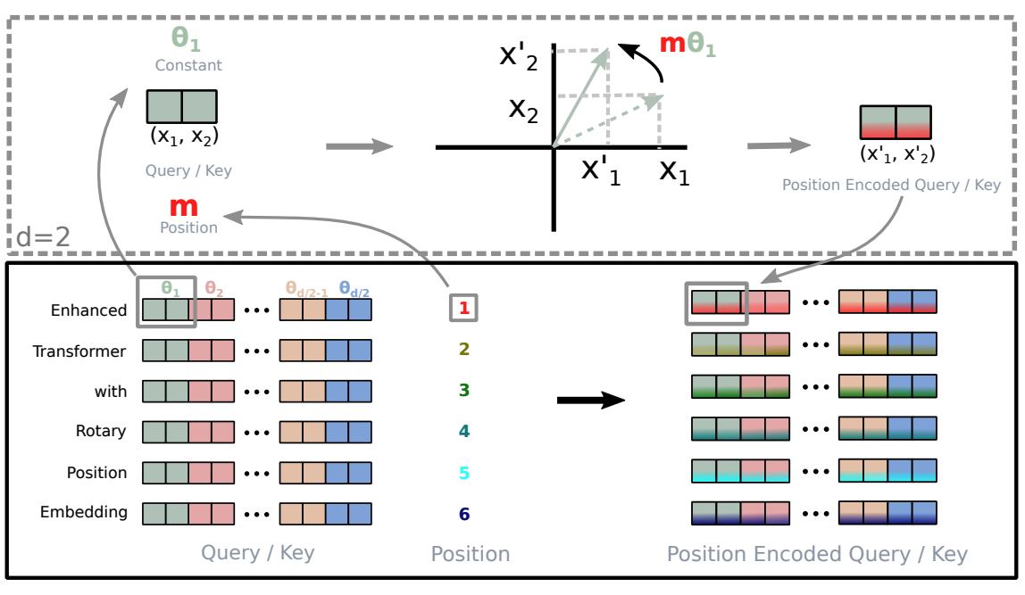
Here’s a subtlety that surprises people: attention as described above is completely permutation-invariant, i.e. it has no built-in notion of token order. If you shuffle a sentence’s words, the attention score between any two given tokens will stay unchanged. So the model needs positional information handed to it explicitly. The most widely used scheme in modern LLMs is Rotary Positional Embeddings (RoPE) (Su et al., 2021), and its idea is elegant: instead of adding a positional signal to the embedding, it rotates the query and key vectors by an angle proportional to their position, before the dot product is taken. Treating each pair of dimensions in $q$ and $k$ as a 2D coordinate, a token at position $m$ gets rotated by:

The beauty of this construction is that the dot product between a rotated query at position $m$ and a rotated key at position $n$ depends only on the relative distance $(m-n)$, not on absolute positions: this is a clean idea to measure “how far apart are these tokens”, directly implemented into attention, rather than learned indirectly from absolute position embeddings. This matters a lot for long-context models: RoPE turns out to be way better suited to interpolation tricks (like “NTK-aware scaling” or “YaRN”) than absolute embeddings are when extending a model trained on short sequences to much longer ones. This partially explains why context windows have grown from a couple thousand tokens to hundreds of thousands or millions.

Act II — Teaching a Transformer

The basic training objective for a language model is actually pretty simple: next-token prediction. Given a sequence $x_1, \ldots, x_n$, the model is trained to predict $x_2$ from $x_1$, $x_3$ from $x_1,x_2$, and so on up to $x_n$ from everything before it. All of this happens in a single forward pass, thanks to the causal mask. The loss is (almost universally) cross-entropy,

and training updates the weights $\theta$ via gradient descent. In practice, almost always with AdamW (Adam with decoupled weight decay), chosen for its robustness to the noisy loss landscapes these models produce. AdamW tracks a running mean $m_t$ and running variance $v_t$ of the gradient $g_t = \nabla_\theta \mathcal{L}$, and uses them to adapt the effective step size per parameter:

where $\hat{m}_t, \hat{v}_t$ are bias-corrected versions of $m_t, v_t$; $\eta$ is the learning rate, and $\lambda\theta_{t-1}$ is the “decoupled” weight decay term that gives AdamW its name, which is applied directly to the weights rather than folded into the gradient the way plain Adam with $L_2$ regularization would do it, which turns out to generalize noticeably better in practice (Loshchilov & Hutter, 2017).

Today’s assistants are built through a sequence of distinct stages layered on top of this objective. Pretraining trains on a huge, broad corpus purely on next-token prediction, and is where the vast majority of compute goes and where the model acquires its raw knowledge of language, facts, and reasoning patterns. Supervised fine-tuning (SFT) then continues training on curated instruction and response examples, teaching the model the format of being a helpful assistant rather than just continuing arbitrary text. Finally, preference tuning shapes the model’s answers toward what humans actually prefer.

The classic approach to that last stage is RLHF (Reinforcement Learning from Human Feedback). Humans rank multiple outputs, a separate reward model $r_\phi(x,y)$ is trained to predict those rankings, and the language model $\pi_\theta$ is optimized (typically via PPO) to maximize that reward, while a KL penalty keeps it from drifting too far from the original SFT model $\pi_{\text{ref}}$ (Ouyang et al., 2022):

The KL term actually matters more than it might look: without it, the model would happily learn to exploit any quirk of the reward model rather than actually getting better (a failure mode usually called “reward hacking”). RLHF works, but it’s a bit awkward, because you’re training and maintaining an entire second model plus an RL loop with well-known stability issues. This motivated simpler alternatives like DPO (Direct Preference Optimization, Rafailov et al., 2023): it shows that the same optimal solution to the objective above can be reached without ever training a reward model or running RL, by reparameterizing the reward directly in terms of the policy itself and optimizing a simple pairwise loss on a preferred response $y_w$ and a dispreferred response $y_l$:

where $\sigma$ is the logistic sigmoid. In simple words, we push the model’s relative preference for the chosen response over the rejected one to be as large as possible, measured relative to what the reference model already thought. IPO adds regularization to this same loss to prevent it from overfitting and pushing probabilities to extremes when preferences are close to deterministic, and KTO (Kahneman-Tversky Optimization) drops the need for paired preference data altogether, learning instead from unpaired binary signal (“this response was good/bad”), which is often much cheaper to collect at scale. The common thread between all of these is that pretraining gives the model capability and this final stage gives it alignment with what people actually want. This is actually important to understand, since a lot of what feels like “the model’s personality” is really a consequence of preference tuning.

Full fine-tuning of a modern LLM (i.e. updating every parameter) is excessively expensive for most use cases, which has spawned a family of much cheaper alternatives. LoRA (Low-Rank Adaptation, Hu et al., 2021) freezes the original weight matrix $W \in \mathbb{R}^{d_{\text{out}} \times d_{\text{in}}}$ and instead learns a low-rank update, so the effective weight used at inference becomes:

The number of trainable parameters drops from $d_{\text{in}} \cdot d_{\text{out}}$ down to $r(d_{\text{in}} + d_{\text{out}})$. For a $4096 \times 4096$ matrix and a moderate rank $r=8$, that’s a reduction from roughly 16.7 million parameters to about 65,000 (over two orders of magnitude smaller), since the update is constrained to a low-dimensional subspace. At inference, $BA$ can even be merged back into $W$ for zero added latency. QLoRA (Dettmers et al., 2023) combines LoRA with 4-bit quantization of the frozen base model, letting you fine-tune tens-of-billions-of-parameters models on a single consumer GPU. And prefix/prompt tuning goes further still, leaving the model’s weights untouched entirely and instead learning a small set of continuous “virtual tokens” prepended to every input. This is cheaper than LoRA, but generally less expressive.

None of this would if we didn’t also have a set of engineering tricks that make training at this scale feasible in the first place. Here is a few of the most notable ones: Mixed precision training performs most computation in 16-bit floating point instead of 32-bit, roughly halving memory use and often doubling throughput on modern tensor cores, while keeping a 32-bit master copy of weights to avoid instability. Gradient checkpointing discards most intermediate activations from the forward pass (which backpropagation would normally need to keep around) and recomputes them on the fly during the backward pass, trading extra compute for a large reduction in peak memory. Sharding (as in ZeRO/FSDP-style parallelism) splits weights, gradients, and optimizer states across many GPUs so no single one needs a full copy of everything, which matters a lot once you remember that AdamW’s momentum and variance terms roughly triple the effective memory footprint of the weights alone. Learning rate schedules typically warm up linearly from near zero over the first steps, to avoid destabilizing the randomly-initialized model with large early updates, and then decay over the rest of training, which empirically beats a constant rate. The most common choice is cosine decay ; it shrinks the learning rate smoothly from a peak $\eta_{\max}$ down to a floor $\eta_{\min}$ following one arc of a cosine curve over the remaining $T$ steps:

A simpler linear decay schedule is sometimes used instead, ramping $\eta_t$ down in a straight line from $\eta_{\max}$ to $\eta_{\min}$ over the same span. And the composition of the training data itself matters as much as any of these: the mixture of web text, books, code, and papers affects downstream capabilities in ways you can measure, while deduplication of near-identical documents avoids wasting compute on redundant signal and reduces the risk of the model simply memorizing evaluation data it happened to see during pretraining (we’ll talk about this shortly).

Act III — Making Generation Fast

From logits to text

At inference time, the model receives a prompt and outputs a probability distribution over the next token, one step at a time, and the real design decison is how you turn that distribution into an actual chosen token. Greedy decoding always picks the single most likely token: it is deterministic, but prone to repetitive text and therefore less creative. Sampling instead draws randomly from the distribution, and temperature $T$ rescales the logits before the softmax, $P(x_i) \propto \exp(z_i/T)$, so that $T<1$ sharpens the distribution toward greedy-like behavior and $T>1$ flattens it toward more randomness. Top-k sampling restricts sampling to only the $k$ most likely tokens, discarding the long tail, while top-p (nucleus) sampling (Holtzman et al., 2019) restricts it instead to the smallest set $V_p$ of tokens whose cumulative probability exceeds a threshold $p$:

This technique allows dynamic adaptation to the shape of the distribution (few tokens when the model is confident, many when it’s uncertain) in a way top-k’s fixed cutoff cannot. Beam search takes a different approach entirely: rather than committing to one token at a time, it maintains the $B$ most promising partial sequences at every step, scoring each candidate sequence by its cumulative log-probability,

often divided by a length-normalization factor $t^\alpha$ (for some $\alpha \in [0,1]$) so that shorter sequences aren’t unfairly favored just for accumulating fewer negative log-probabilities, then expanding each surviving candidate and keeping only the overall top $B$ by this score. This tends to find higher joint-probability sequences than greedy decoding, but is less common for open-ended chat (where diversity matters and there’s no single correct continuation) than for tasks like translation, where a single best answer exists.

Generation is also sequential by nature (token $n+1$ needs token $n$) which makes a single GPU largely latency-bound rather than throughput-bound, often sitting mostly idle while waiting on this chain. Speculative decoding (Leviathan et al., 2023; Chen et al., 2023) exploits exactly this: a small, fast “draft” model proposes several tokens ahead, and the large “target” model verifies all of them in a single parallel forward pass, accepting whatever prefix matches what it would have generated itself. Because verifying several tokens at once costs barely more than verifying one (the bottleneck here is memory bandwidth, not compute), this yields substantial speedups while producing an output distribution mathematically identical to standard sampling from the target model; it’s a pure efficiency trick, with no approximation.

KV cache and cache-shrinking tricks

Generating each new token in theory requires recomputing attention over the entire previous context from scratch, which means recomputing every key and value vector for every earlier token, at every single step. This is highly wasteful since those earlier keys and values never change. The KV cache fixes this for us: for each previous token, the model stores its key and value vectors once, and when generating a new token, only needs to compute the new token’s own query (and key/value), comparing it against the already-cached keys of everything before it. This turns an $O(n^2)$-per-step problem into $O(n)$-per-step, and is probably the single most important systems-level optimization that makes autoregressive generation usable at all.

The catch is that the cache’s memory cost grows linearly with sequence length and with the number of concurrent requests, and for long-context or high-throughput serving this often becomes the dominant memory bottleneck on the GPU ; this is often even more constraining than the model’s own weights. Concretely, for a sequence of length $n$, the total KV cache size (in bytes) across the whole model is:

(the leading factor of 2 accounts for storing both keys and values). Every term on the right besides $n$ is fixed by the model’s architecture, which is exactly why techniques that shrink $n_{\text{kv_heads}}$ (MQA/GQA, see below) or the “bytes per value” term (cache quantization) act as direct multiplicative discounts on this formula, rather than one-off tricks. This has spawned a whole subfield of cache-shrinking tricks. For example, KV cache quantization stores cached keys and values in lower precision (8-bit or 4-bit instead of 16-bit), trading a little numerical accuracy for a large reduction in memory, which allows serving more users or longer contexts on the same hardware. KV cache eviction selectively discards less-important cached entries for very long contexts rather than keeping the entire history, as in approaches like StreamingLLM (Xiao et al., 2023), which surfaced a curious finding along the way: naively evicting old tokens (say, with a sliding window keeping only the most recent $N$) causes quality to collapse, because the model allocates a disproportionate amount of attention to the very first few tokens of a sequence regardless of their content, using them as a dumping ground for “unused” softmax mass. These attention sinks need to be kept in the cache permanently, no matter how far a sliding window moves past them, for quality to hold up. And at the architecture level, multi-query attention (MQA) and grouped-query attention (GQA) (Shazeer, 2019; Ainslie et al., 2023) shrink the cache directly by sharing a single K/V pair across all heads (MQA) or across groups of heads (GQA) (while queries stay per-head) with GQA now the standard choice in models like LLaMA 2/3 and Mistral, since it captures most of MQA’s memory savings while preserving much more of full multi-head attention’s quality.

The generation loop, in pseudocode

All of the pieces above (causal mask, decoding strategies, the KV cache…) fit together into one loop, and it’s worth seeing that loop written out explicitly, since a lot of the vocabulary (prefill, decode step, cache) refers directly to pieces of it.

Generation happens in two distinct phases. First, a prefill phase processes the entire input prompt in one parallel forward pass, populating the KV cache for every prompt token at once. Then a decode phase generates new tokens one at a time, each step reusing the cache instead of recomputing it. Alltogether it looks something like this:

def GENERATE(prompt_tokens, max_new_tokens):
    # --- Prefill phase: one parallel pass over the whole prompt ---
    kv_cache = empty_cache()
    logits, kv_cache = model.forward(prompt_tokens, kv_cache)
    # logits here only matters for the LAST position — that's our first prediction

    generated = []
    next_token = sample(logits[-1])   # greedy / top-k / top-p / temperature

    # --- Decode phase: one new token per step, reusing the cache ---
    for step in range(max_new_tokens):
        generated.append(next_token)

        if next_token == END_OF_SEQUENCE:
            break

        # Only the ONE new token is run through the model.
        # Its query attends to every cached key/value from all previous tokens.
        logits, kv_cache = model.forward(next_token, kv_cache)
        next_token = sample(logits[-1])

    return generated

A few details map directly onto earlier sections. Inside model.forward, each transformer block runs attention using the new token’s freshly computed query against the cached keys and values of every earlier token, plus the new token’s own freshly computed key and value, which then get appended to the cache for the next step: this corresponds to the $O(n)$-per-step saving from the KV cache section above, instead of recomputing all $n$ keys and values from scratch on every single step. The sample(...) call is where greedy decoding, temperature, top-k, or top-p actually get applied: it’s basically a choice of how to turn the final logits into a token, completely separate from the model’s forward pass itself. And speculative decoding modifies this loop by having a small draft model run several iterations of the decode loop ahead of time, then verifying the whole proposed chunk with a single call to the large model’s forward, rather than one call per token.

Beam search departs from this loop more than the others, since it isn’t tracking a single sequence: instead of one generated list, it maintains $B$ candidate sequences (and $B$ KV caches) in parallel, expands each by its most likely next tokens, and prunes back down to the $B$ best sequences overall by cumulative log-probability at every step (which is also why it’s more expensive per step than simple sampling, by roughly a factor of $B$).

Rethinking attention itself

Standard (“dense”) attention scores every pair of tokens, costing $O(n^2)$ in compute and memory as sequence length grows ; this is the root cause of both the KV cache’s exploding cost and the rising per-token attention cost as the context windows stretches out. Several architectural approaches trade off the “completeness” of attention for tractable alternatives. For instance, sliding window attention restricts each token to a fixed-size window of recent tokens rather than the full history, capping cost at $O(w)$ instead of $O(n)$ (used in Mistral 7B, among others) at the cost of losing very-long-range dependencies directly, though stacked layers can still propagate information further back indirectly, since a token two layers deep effectively sees roughly $2w$ tokens behind it. Alternatively, a sliding window with recomputation periodically runs a fuller attention pass over a longer span, trading extra compute to recover some of the long-range dependencies a pure window would miss. Sparse attention patterns (Sparse Transformer, Child et al., 2019; BigBird, Zaheer et al., 2020) attend to a structured subset of positions (local, strided, global) chosen so information can still propagate across the whole sequence within a few layers, while each individual computation stays cheap.

FlashAttention (Dao et al., 2022) is different from everything above: it isn’t an approximation. Instead, it computes mathematically exact standard attention, just far faster. The insight is about hardware, not the math behind it: on a GPU, attention’s bottleneck is usually not the arithmetic itself but moving data between slow high-bandwidth memory (HBM) and the much faster on-chip SRAM, and naive implementations materialize the full $n \times n$ score matrix in HBM, then read it back twice more: once for the softmax, once for the weighted sum. FlashAttention instead tiles the computation into blocks small enough to fit in fast on-chip memory, computing a running, numerically stable softmax incrementally and never materializing the full matrix in slow memory at all. The output is bit-for-bit equivalent to standard attention, just much faster and more memory-efficient. Thi is why it was adopted almost universally within about a year of release, with no real quality tradeoff to weigh against the speedup.

From one request to millions

Everything above is about a single forward pass, but serving a model to many users simultaneously introduces its own set of problems. A naive server allocates a large, contiguous chunk of GPU memory per request for its KV cache, sized for the maximum sequence length the request might reach ; this is wasteful, since most requests are much shorter than that worst case. PagedAttention (Kwon et al., 2023) borrows a decades-old idea from operating systems: virtual memory paging. This is actually the core idea behind the popular vLLM serving engine. The KV cache is split into fixed-size pages allocated on demand, with a lookup table mapping each request’s logical positions to wherever they physically sit in GPU memory, which eliminates most memory fragmentation and allows a server pack far more concurrent requests into the same hardware.

Traditional batching waits for an entire batch of requests to all finish before starting a new one, leaving the GPU partially idle whenever any single request finishes early while others run long. We can instead use continuous batching to add new requests into a running batch and remove finished ones dynamically at each generation step, keeping the utilization consistently high. Another idea is prefix caching: it exploits the fact that many requests share a common prefix, like a system prompt, a repeatedly-queried document, a few-shot template… It stores and reuses the KV cache for that shared prefix across different requests, skipping its recomputation entirely. And when a model is too large to fit on a single GPU, or if you simply want more throughput, you can split it across several GPUs: tensor parallelism splits individual weight matrices within a layer across GPUs, keeping latency low at the cost of needing fast interconnects (since communication happens at every layer), while pipeline parallelism assigns different layers to different GPUs like an assembly line, communicating less often but risking idle “bubbles” unless carefully scheduled. These same two strategies, alongside data parallelism (replicating the whole model and splitting the training data), also underpin distributed training of large models, not just serving.

Act IV — Living With a Fixed Window

Longer context windows sound like a great idea, but they come with real costs that don’t disappear just because the model accepts more tokens as input. First of all, attention cost and KV cache size both grow with context length, but there’s also a third, more subtle issue: information placed in the middle of a long context tends to be underused. This “lost in the middle” effect (Liu et al., 2023) is a widely-replicated finding that models use information at the very beginning or very end of a long context noticeably better than information buried in the middle, producing a U-shaped accuracy curve as a function of where the relevant fact sits. This is a genuine and unresolved quality limitation, and it’s exactly why practical advice like “put your most important instructions at the start or end of a long prompt” exists.

To measure whether a model’s context window actually works, rather than just accepting a large number of input tokens, we needed to come up with some new techniques. Needle-in-a-haystack testing buries a specific / distinctive fact somewhere within a very long context and checks whether the model can retrieve it, varying both the context length and the needle’s position: this is a direct probe of the lost-in-the-middle effect. More broadly, perplexity (the exponential of the average cross-entropy loss, $\text{PPL} = \exp(\mathcal{L})$) measures how surprised, on average, a model is by real text, but says little about instruction-following or reasoning. Finally, benchmark contamination (where public test questions have leaked into the enormous web-scraped corpora used for pretraining) has pushed the field toward held-out, frequently refreshed, or private evaluation sets.

Even with genuinely long context windows, stuffing an entire knowledge base into every prompt is often wasteful and expensive when even possible. This is the problem that Retrieval-Augmented Generation (RAG) (Lewis et al., 2020) solves: instead of relying purely on what the model memorized during pretraining, a retrieval step fetches only the most relevant pieces of external information at query time, and only those go into the prompt. A typical RAG pipeline first chunks large documents into smaller, retrievable pieces (since retrieval systems generally work over a few hundred to a couple thousand tokens at a time), so chunk size and overlap are real design decisions (e.g. too small loses context, too large dilutes relevance). An initial fast, embedding-based retrieval pass then casts a wide net over candidate chunks, and a slower, more accurate reranker re-scores this smaller candidate set for actual relevance, improving precision at a fraction of the cost of running that expensive scoring over the whole corpus. Finally, context compression (via summarization, extraction of the most relevant sentences, or learned compression modules) shrinks the retrieved chunks further before they enter the prompt, both to fit more relevant information into a limited budget and to avoid diluting the prompt with less-relevant surrounding text.

Act V — Bigger and Cheaper at the Same Time

There are two largely independent tricks let you get more out of a model’s parameter budget without paying for it in full at inference time.

Mixture of Experts (MoE): MoEs replace the single, dense MLP in each block with many parallel MLPs (“experts”), plus a small learned router that, for each token, selects only a small subset of experts (just 1 or 2) to actually process it. Formally, given $N$ experts $E_1, \ldots, E_N$ and a router with learned weights $W_r$, the router first scores every expert for token $x$, keeps only the top $k$ scores, and zeroes out the rest before renormalizing with a softmax:

Since $g_i(x) = 0$ for every expert outside the top $k$, the sum on the right only actually needs to evaluate those $k$ experts, not all $N$ ; this sparsity in $g(x)$ is precisely what keeps the active compute per token small even as $N$ grows large. The model’s total parameter count, and thus its knowledge capacity, can be enormous, while the active compute per token, which is what actually determines latency and cost, stays comparable to a much smaller dense model, since each token only passes through a couple of experts rather than one giant shared MLP. Models like Mixtral (Jiang et al., 2024) popularized this at scale. But as always there are trade-offs: MoE models need a lot more total GPU memory, since all experts must be loaded even though only a few are used per token, and training them stably requires auxiliary load-balancing losses to stop the router from collapsing onto always favoring the same few experts.

Quantization: it attacks the same cost problem from the opposite direction. Instead of using fewer parameters per token, it uses fewer bits per parameter. Model weights and activations are typically trained in 16-bit floating point, and quantization compresses this further (commonly to 8-bit or 4-bit) to shrink memory footprint and speed up inference, since moving and multiplying smaller numbers is both faster and cheaper. The simplest version, uniform integer quantization, picks a scale $s$ and zero-point $z$ from the range of values being quantized, and maps each real value $x$ to the nearest representable integer:

for a target bit-width $b$ (e.g. $b=8$ or $b=4$), with the original value recovered approximately at inference time via $x \approx s\,(x_q - z)$. The whole practical difficulty in quantization research is choosing $s$ and $z$ well (per-tensor vs. per-channel scales, handling outlier values…) rather than the mapping itself, which is actuallt quite simple. Weight quantization compresses the static weights, which is generally the easier and lower-risk target since it can be done carefully offline with calibration data (methods like GPTQ, Frantar et al., 2022, and AWQ, Lin et al., 2023, are specifically designed to minimize the resulting accuracy loss). On the other side, activation quantization quantizes the activations flowing through the network at inference time ; this is harder because activations vary per-input and can contain occasional large outlier values that are disproportionately important, making naive schemes prone to sharper accuracy drops. QLoRA, mentioned earlier, sits at the intersection of both worlds: it combines 4-bit weight quantization of a frozen base model with LoRA fine-tuning of a small set of full-precision adapter weights, getting most of the memory savings of aggressive quantization during fine-tuning while still letting the model adapt through the unquantized LoRA parameters.

Act VI — Peeking Inside, and Using It Well

A separate and increasingly active research direction is about “what is actually happening inside them?” (mostly referred to as mechanistic interpretability — see this blog’s introduction to the field for a much deeper tour). In that end, logit lens (nostalgebraist, 2020) is a useful tool that takes the residual stream’s state $x^{(l)}$ at an intermediate layer $l$ and passes it directly through the model’s final normalization and unembedding matrix $W_U$, as if that layer were already the output:

Note that $W_U$ was only ever trained to be applied to the final layer’s output, $x^{(L)}$. For $l < L$, $\hat y^{(l)}$ can often be useful enough to reveal a rough, evolving “guess” at the model’s eventual prediction building up gradually across layers, suggesting the residual stream accumulates evidence toward an answer progressively rather than computing it only at the very end. Another method for analysing the model is activation patching (or causal tracing): it runs the model on two different inputs, then patches an internal activation from one run into the other at a specific layer and position, observing how the output changes ; this lets researchers make causal claims about which components are responsible for a specific behavior, rather than just noticing correlations. Attention head analysis directly inspects what specific heads attend to across many examples, which can reveal specialized, human-interpretable roles, such as heads that consistently attend to the previous occurrence of the current token (“induction heads,” Olsson et al., 2022, believed to be a major mechanistic contributor to in-context learning — see this blog’s post on in-context learning for more on both). And because individual neurons are frequently polysemantic (a single neuron firing for several unrelated concepts, making direct neuron-level interpretation unreliable), we train sparse autoencoders (SAEs) to reconstruct a layer’s activations as a sparse combination of a much larger set of learned “feature” directions, under the hypothesis that these directions correspond to cleaner, more monosemantic concepts than the raw neurons do (Bricken et al., 2023, and its follow-up “Scaling Monosemanticity” work, are the most prominent examples applied at scale).

The final layer of this whole stack is actually how you phrase what you ask the model. Chain-of-thought (CoT) prompting (Wei et al., 2022) is about asking the model to reason step by step before giving a final answer, and improves performance on tasks requiring multi-step reasoning, plausibly because it gives the model’s fixed per-token compute budget more intermediate “thinking space” and more closely follows the patterns of solved problems seen during training. Few-shot prompting includes a small number of worked examples directly in the prompt, letting the model infer the desired task and format without any weight updates, exploiting the in-context learning capability that emerges from large-scale pretraining. Similarly, system prompts provide a separate instruction channel, typically set once by a developer or platform rather than the end user, establishing persistent behavior, tone, or constraints across an entire conversation. None of these change the model’s weights at all, and they’re entirely a matter of how information is arranged within an input the model already knows how to process, which says a lot about how much capability gets packed into the pretraining and fine-tuning stages described earlier.

One distinction that’s easy to gloss over: not every transformer is built the same way internally. Encoder-only models (like BERT) see the whole input bidirectionally, with every token attending to every other and no causal mask, which is good for tasks like classification where the full input is available upfront. Decoder-only models generate left to right with the causal masking described in Act I. This is the architecture behind nearly every modern general-purpose LLM (GPT, Claude…). Encoder-decoder models use both, with an encoder fully processing the input and a separate decoder generating output, attending both to its own previous tokens (causally) and to the encoder’s representations (bidirectionally). This is the dominant architecture for translation-style tasks, and how the original transformer paper itself, along with T5, was built. When people casually say “LLM” today, they almost always mean a large decoder-only, causal transformer.

Closing Thoughts

If we slow down and take a step back, you can realize that the basic block of Transformer (attention, then an MLP, wrapped in a residual stream) is still exactly what’s running underneath all the sections of this post. Nothing in RLHF, MoE, FlashAttention, or RAG changes that block; each one just makes it cheaper to train, to serve, or better matched to the task we are excecuting. Once you see that block clearly, the rest of the field is about optimization and tricks: RoPE and GQA are opinions about how attention should be computed, LoRA and quantization discuss how much of the model actually needs to move or stay at full precision, and RAG / long-context tricks care about how much of the answer should live in the weights versus the prompt. None of that requires inventing a new primitive, which is itself the more interesting fact: an idea this simple turned out to have this much room in it.

References

• Vaswani, A. et al. (2017). Attention Is All You Need. NeurIPS.
• Su, J. et al. (2021). RoFormer: Enhanced Transformer with Rotary Position Embedding. arXiv:2104.09864.
• Shazeer, N. (2020). GLU Variants Improve Transformer. arXiv:2002.05202.
• Xiong, R. et al. (2020). On Layer Normalization in the Transformer Architecture. ICML.
• Zhang, B., & Sennrich, R. (2019). Root Mean Square Layer Normalization. NeurIPS.
• Loshchilov, I., & Hutter, F. (2017). Decoupled Weight Decay Regularization. arXiv:1711.05101.
• Ouyang, L. et al. (2022). Training Language Models to Follow Instructions with Human Feedback. NeurIPS.
• Rafailov, R. et al. (2023). Direct Preference Optimization: Your Language Model Is Secretly a Reward Model. NeurIPS.
• Hu, E. J. et al. (2021). LoRA: Low-Rank Adaptation of Large Language Models. arXiv:2106.09685.
• Dettmers, T. et al. (2023). QLoRA: Efficient Finetuning of Quantized LLMs. NeurIPS.
• Holtzman, A. et al. (2019). The Curious Case of Neural Text Degeneration. arXiv:1904.09751.
• Leviathan, Y., Kalman, M., & Matias, Y. (2023). Fast Inference from Transformers via Speculative Decoding. ICML.
• Chen, C. et al. (2023). Accelerating Large Language Model Decoding with Speculative Sampling. arXiv:2302.01318.
• Shazeer, N. (2019). Fast Transformer Decoding: One Write-Head Is All You Need. arXiv:1911.02150.
• Ainslie, J. et al. (2023). GQA: Training Generalized Multi-Query Transformer Models from Multi-Head Checkpoints. EMNLP.
• Xiao, G. et al. (2023). Efficient Streaming Language Models with Attention Sinks. arXiv:2309.17453.
• Dao, T. et al. (2022). FlashAttention: Fast and Memory-Efficient Exact Attention with IO-Awareness. NeurIPS.
• Kwon, W. et al. (2023). Efficient Memory Management for Large Language Model Serving with PagedAttention. SOSP.
• Lewis, P. et al. (2020). Retrieval-Augmented Generation for Knowledge-Intensive NLP Tasks. NeurIPS.
• Liu, N. F. et al. (2023). Lost in the Middle: How Language Models Use Long Contexts. arXiv:2307.03172.
• Jiang, A. Q. et al. (2024). Mixtral of Experts. arXiv:2401.04088.
• Frantar, E. et al. (2022). GPTQ: Accurate Post-Training Quantization for Generative Pre-trained Transformers. arXiv:2210.17323.
• Lin, J. et al. (2023). AWQ: Activation-aware Weight Quantization for LLM Compression and Acceleration. arXiv:2306.00978.
• Wei, J. et al. (2022). Chain-of-Thought Prompting Elicits Reasoning in Large Language Models. NeurIPS.
• nostalgebraist. (2020). Interpreting GPT: The Logit Lens. LessWrong.
• Olsson, C. et al. (2022). In-context Learning and Induction Heads. Transformer Circuits Thread, Anthropic.
• Bricken, T. et al. (2023). Towards Monosemanticity: Decomposing Language Models with Dictionary Learning. Transformer Circuits Thread, Anthropic.